State Variables, Phase Space, and Trajectories

Since the study of nonlinear dynamics is very qualitative, there are many terms used to identify specific concepts.

State Variables

A state variable is a variable of a system of ODEs. These represent different quantities and usually rely on the other state variables of the system. They represent some aspect of the system we are modelling. For example, in the case of a swinging pendulum, we need the angle of the pendulum and its velocity to determine where the pendulum will go next. As shown in previous sections, the system of ODEs for the pendulum is

\begin{align} \dot{\omega} &= - \frac{g}{L}\sin(\theta) \\\\ \dot{\theta} &= \omega \end{align}

In that example, \(\theta\) would represent the angle, and \(\omega\) would represent the velocity. These represent the state of the system at any given time, and therefore are called state variables.

Phase Space

This is the space of all state variables, and is therefore also sometimes called the state space. In a 1D system, this is typically just the real line \(\mathbb{R}\) and is sometimes called the phase/state line. In 2D the phase space is sometimes called the phase portrait. The phase space typically does not include the time variable \(t\), as this is an independent variable and does not rely on the state of the system.

Trajectories

A trajectory of a system is simply a parametric curve that satisfies the system of ODEs. These are sometimes also called solution curves. Note that these are curves in the phase space and not in some other space, such as a physical space. Using the pendulum example again

\begin{align} \dot{\omega} &= - \frac{g}{L}\sin(\theta) \\\\ \dot{\theta} &= \omega \end{align}

The trajectories would be the parametric curves \((\omega(t), \theta(t))\) or \((\theta(t), \omega(t))\) depending on how you want to visualize it. From this, you can deduce the physical evolution given a starting velocity \(\omega(0)\) and a starting angle \(\theta(0)\). Now from our uniqueness theorem, we can deduce another interesting fact about these trajectories. That is, no curves in phase space can intersect. This is not an insignificant result. That means, given any two initial conditions in phase space, if at any point in time the curves intersect each other, they must be the same curve. This means that the second initial condition is simply the evolution of the first. This might be confusing now but will make more sense visually in later sections. We can also deduce several results from this.

Examples

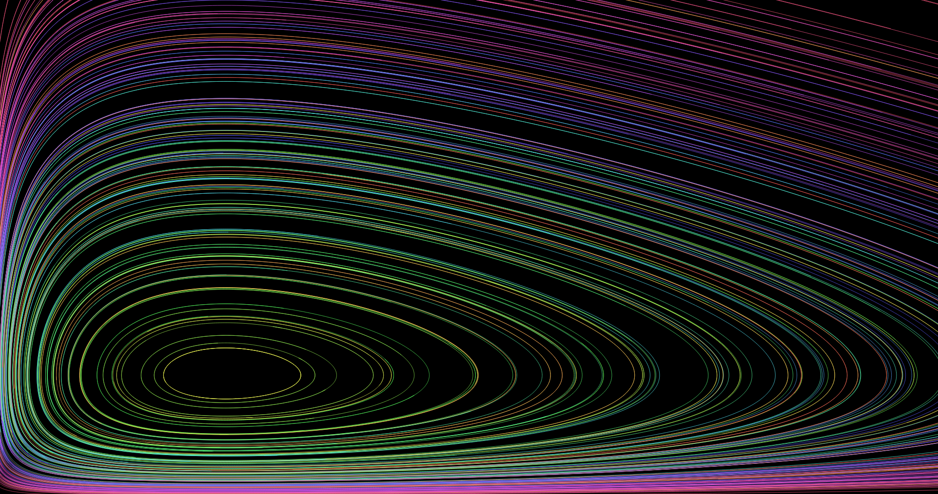
Consider the Lotka-Volterra Equations that govern certain competitive populations.

\begin{align} \dot{x} &= \alpha x - \beta xy \\\\ \dot{y} &= -\gamma y + \delta xy \end{align}

Here, \(x\) is the population of rabbits, and \(y\) is the population of foxes (although this can model more than just foxes and rabbits). The values \(\alpha, \beta, \gamma, \delta\) are parameters and are constant here. Parameters are one of (if not) the most important consideration of dynamical systems, as they can qualitatively change system dynamics. But for now, we are more interested in the trajectories in phase space.

Now in this example, the phase space is 2D and therefore we can refer to it as the phase portrait. Another consideration in visualizing the space is the realistic interpretation of the values. Populations cannot be negative and therefore we can consider the upper right plane of the system, that is \(x > 0\) and \(y > 0\). Now below is an example of the phase portrait with representative trajectories as different colors, notice how none of them intersect.

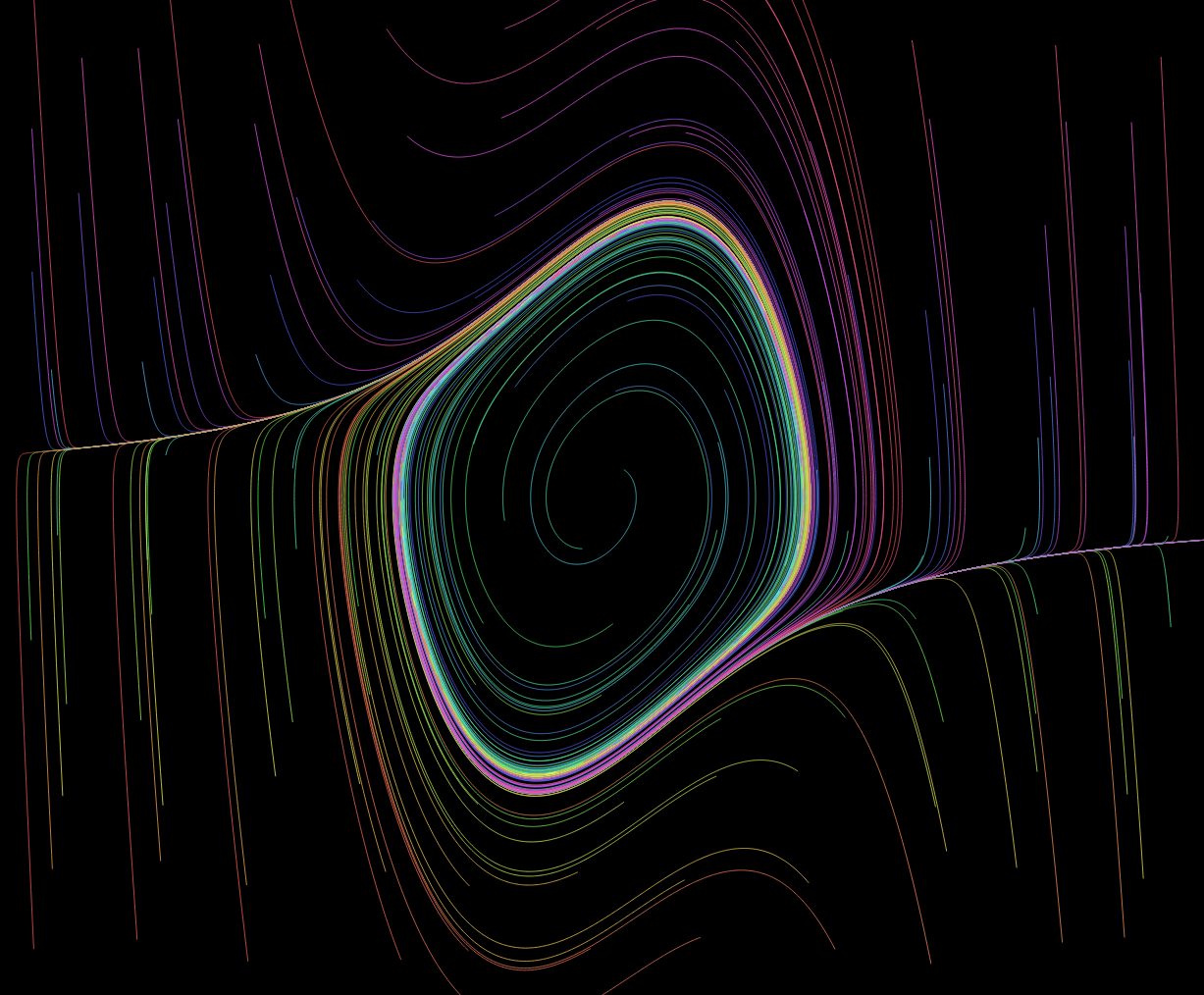
lotka-volterra — Lotka–Volterra phase portrait

Here is an example of the phase portrait of the Van der Pol Oscillator which models systems with self-sustained oscillations (occurs in biology, physics, and engineering). It's actually a special case of the system below it.

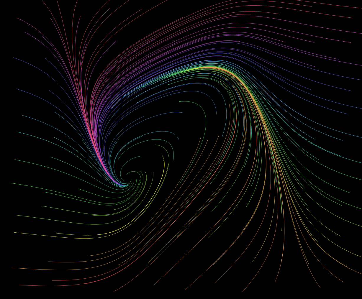
Here is an example of the phase portrait of the FitzHugh-Nagumo model which is a simplified model of the voltage and gating mechanics of a neuron.

You can experiment with my phase portrait simulation here. If it looks like any of these curves intersect, it's because they get infinitesimally close, but never touch. We will learn how to derive these portraits to determine the nature of the systems. Note that the simulation I linked evolves in real time. Typically we do not have that, and instead we have a static graph with lines along the curve that tell you how it will evolve in time. This leads into the final topic of this section.

Vector Fields

2D (and even 1D with some changes) systems essentially represent a vector field. At each point on the phase plane we draw a vector that represents the magnitude of change determined by the corresponding ODE. In that sense, we can interpret a phase portrait as a vector field, depending on how we draw it. Each vector tells us how we are going to change with a small step in time, and therefore we can follow these vectors to see how we would evolve in time starting at various states. I will go into more detail on this in the relevant sections.