One Dimensional Systems

Now that we have shown that any higher order ODEs can be reduced into a system of first order ODEs, the ability to analyze first order ODEs is obviously important. The first step in this process is fixed point analysis.

Fixed Point Analysis

As mentioned, we can analyze systems of autonomous first order ODEs individually at first. We begin with the aforementioned fixed point analysis.. First let's consider such a system,

\dot{x} = f(x)

The fixed points, are the points \(x^*\) such that

\[ f(x^*) = 0 \]

Since the right hand side of these systems are algebraic, it is often pretty straightforward to find these points. It's not always easy to find it analytically, but numerical approximations can work as well.

Now what does it mean for our system when \(f(x) = 0\)? This means that our state variable \(x\) is not changing. That is, the derivative (instantaneous rate of change) is \(0\) and will stay \(0\). Since,

\dot{x} = f(x^*) = 0

Finding this point is simply finding the value of \(x\) at which the state will never move. This is why it's called a fixed point. Due to our uniqueness and existence theorems, we know that no other trajectory can ever intersect the fixed point. This is due to the fact that there is a trajectory starting at the fixed point and stays there forever, and if some other trajectory intersected this point it would contradict the uniqueness of solutions that we have. However, fixed points dominate the behavior of any system but especially 1D systems. In one dimension, each trajectory will either get arbitrarily close to a fixed point, or go off to infinity. Now let's consider a concrete example.

Examples

Consider the 1D system called the Logistic Equation which models the population dynamics of a single species.

\dot{x} = rx(1-\frac{x}{L})

Where \(x(t)\) is the population of the species at time \(t\), \(r\) is the reproduction rate, and \(L\) is the carrying capacity. \(r\) and \(L\) are both constants. Now let's find when the population stops changing. This happens when

rx(1-\frac{x}{L}) = 0

Rearranging for \(x\), we get

-\frac{x^2}{L} + x = 0

This is a quadratic equation in \(x\), with \(a = -\frac{1}{L}, b = 1, c= 0\). The quadratic equation is.

\frac{-b \pm \sqrt{b^2-4ac}}{2a}

With our values we get

\frac{(-1 \pm \sqrt{1})}{-2/L}

\(L\) is a free parameter and so we will let \(L = 100\) for simplicity. Then we have two fixed points

\begin{align} x_1 &= \frac{(-1 + 1)}{-2/100} = 0 \\\\ x_2 &= \frac{(-1-1)}{-2/100} = 100 \end{align}

Now let's interpret this. If the population is originally at \(0\), then it will never grow. This makes sense and is physically accurate. On the other hand, if the population is at \(100\) (its carrying capacity), then it won't grow (or shrink), the population will remain at that value forever.

What about other values? There are two important regions to consider, populations between \(0\) and \(100\) and populations greater than \(100\). To understand them, we must understand the right hand side of the ODE, i.e.

rx(1-\frac{x}{100})

Now let's take \(r=1.25\). In other words the population grows by a quarter of its current population. Choosing different values of \(r\) will change the dynamics. We will discuss that later. Subbing \(1.25\) in, we have

1.25x(1-\frac{x}{100})

This is a concave down parabola with zeros at \(x=0\) and \(x=100\) (as previously found).

logisticCurve — \(1.25x(1-x^2)\) Graphed

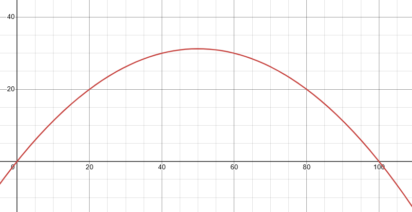
This curve is itself what dictates the population change. So when this curve is negative, we have population loss, conversely when it is positive, we have population growth. In 1D it is useful to plot \(x\) vs. \(\dot{x}\). Where \(\dot{x}\) is given by the curve above. Doing so, we have the following graph.

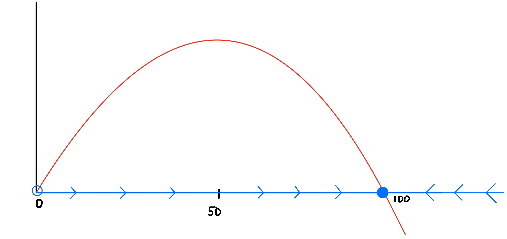
The blue line represents the actual population. The arrows are vector arrows, it tells you where the population will move in time. Notice the two circles at \(x=0\) and \(x=100\). As we can see for the one at \(x=0\), all arrows point away from it. We say that this fixed point is unstable, we also sometimes call it a source. We denote this graphically with the empty circle as shown in the image. Now consider the fixed point at \(x=100\). All arrows near it are pointing towards it. We call this fixed point stable and in some contexts, attracting. These fixed points are denoted graphically with filled in circles as shown. Now we can deduce the fundamental nature of the entire system as follows: if the population is above \(100\), the population will decline to \(100\) (technically will get arbitrarily close and never touch it). If the population is greater than \(0\) but less than \(100\), then it will grow to \(100\) (similarly arbitrarily close but not exactly \(100\)). If the populations start at either of the fixed points \(0\) or \(100\), then they will remain there forever. The rate of growth at a certain population can be deduced by taking the derivative of the right hand side with respect to \(x\) (not \(t\)). We can see this graphically as well. The slope of the curve above is the speed at which the population is changing. This peaks near the beginning and decreases until around \(x=50\) (middle of the parabola) and then becomes negative, causing a decreased rate as it approaches \(100\). More quantitatively, we can inspect how fast the population will change with respect to the current population by taking the derivative of it with respect to \(x\). In our example, if

f(x) = 1.25x(1-\frac{x}{100})

Then, we can find the rate of change of this function by computing

\frac{df}{dx} = r(1-\frac{2x}{L})

This leads us to the final step in this level of analysis. Linearization.

Linearization and Fixed Point Stability

Although we can see all of this graphically, we need a way to mathematically deduce these results. This is where linearization is used. The idea is that we want to see what would happen to a trajectory that starts very close to a fixed point. Does it grow further away? Does it grow closer? Can we not tell? We can answer these with linearization. First, as mentioned, consider a small perturbation near a fixed point. First, let's consider a general first order autonomous ODE.

\dot{x} = f(x)

Let,

x = x^*+\eta(t)

Where \(x^*\) is a fixed point and \(\eta\) is a small perturbation near the fixed point. Then,

\dot{x} = \dot{\eta}(t)

Since \(x^*\) is a fixed point, its derivative is \(0\). Furthermore, since

\dot{x} = f(x),

we get

\dot{\eta}(t) = f(x) = f(x^* + \eta(t)).

Therefore, we have

\dot{\eta}(t) = f(x^* + \eta(t)).

Now we linearize using a Taylor expansion of \(f\) about \(x^*\):

f(x^* + \eta) \approx f(x^*) + f'(x^*)\eta + \mathcal{O}(\eta^2).

But \(f(x^*) = 0\) since \(x^*\) is a fixed point. Ignoring higher-order terms gives

\dot{\eta}(t) \approx f'(x^*) \eta(t).

Note that for the \(x-x^*\) term in the Taylor expansion, we get that

x = x^* + \eta(t) \implies \eta(t) = x-x^*

Now back to

\dot{\eta}(t) \approx f'(x^*) \eta(t).

This is a linear differential equation whose solution is

\eta(t) = \eta(0) e^{f'(x^*) t}.

Finally:

If \(f'(x^*) < 0\), then \(\eta(t) \to 0\) and the fixed point is stable.
If \(f'(x^*) > 0\), then \(\eta(t)\) grows and the fixed point is unstable.

A hyperbolic fixed point is a fixed point where \(f'(x^*) \neq 0\). If \(f'(x^*) = 0\), the point is called non-hyperbolic, and higher-order terms must be analyzed to determine stability. So as long as the point is hyperbolic, we can quantitatively determine its stability. Let's try it for our example above.

Linearization of the Logistic Equation

This is pretty straightforward; we already have the expression for the linearization, we just need to compute the necessary derivatives for each fixed point. First let's pre-compute \(f'\), so that we have it for both expressions.

f(x) = 1.25x(1-\frac{x}{100})

\implies f'(x) = 1.25-2.5\frac{x}{100}

Now let's consider \(x^* = 0\)

f'(0) = 1.25 \implies f'(x^*) > 0

Therefore, we have shown that the fixed point \(x^* = 0\) is unstable (aka repelling or a source). Any nearby trajectories grow in time.

Finally, let's consider the fixed point \(x^* = 100\)

\begin{align} f'(100) &= 1.25-2.5 \cdot \frac{100}{100} \\ f'(100) &= -1.25 \implies f'(x^*) < 0 \end{align}

Therefore we see that both fixed points are hyperbolic, and that the second fixed point \(x^* = 100\) is stable (aka attracting or a sink). Any nearby trajectories are pulled towards the fixed point, sort of like a blackhole.

We have now gone over fixed point analysis and linearization for 1D systems. These concepts are extremely important and typically the first steps to analyzing any system. In higher dimensions, we build upon these ideas with things like the Jacobian. Again, the intuition behind linearization is to see what would happen if we started a trajectory very close to a fixed point. If the distance to the fixed point decays, then it's attracting. If the distance to the fixed point grows, then it's repelling. This concludes the preliminary analysis of 1D systems. However, this is not all. I cover dependence on parameters in the next section and how changing parameters can make or break stability. These qualitative changes in the system's behavior are known as bifurcations, and they have very rich and interesting theory.